Benchmarks

This section demonstrates the accuracy, the computation speed and the memory requirements of spherical harmonic analysis and synthesis of point data values. Applied is the Gauss–Legendre quadrature, which offers the best performance. All tests were executed on a PC with the Intel(R) Core(TM) i7-6800K CPU @ 3.40GHz and 128 GBs of RAM. CHarm was compiled using GCC with --enable-openmp, --enable-avx2 and CFLAGS="-O3 -ffast-math" installation flags. All 6 CPU cores were employed with hyperthreading enabled. Polar optimization was disabled unless explicitly stated otherwise.

The benchmarks can be executed by make bench after running ./configure and make. The outputs from the benchmark program (the accuracy and wall-clock times) can be plotted by a Python script plot-bench.py inside the bench folder (requires numpy and matplotlib). The memory requirements can be plotted by the plot-memory.py script that can be found inside the same directory.

Warning

The benchmark program may require up 56 GBs of RAM! Do not execute it if you do not have that much RAM available. Alternatively, modify the nmax_all array inside ./bench/bench.c.

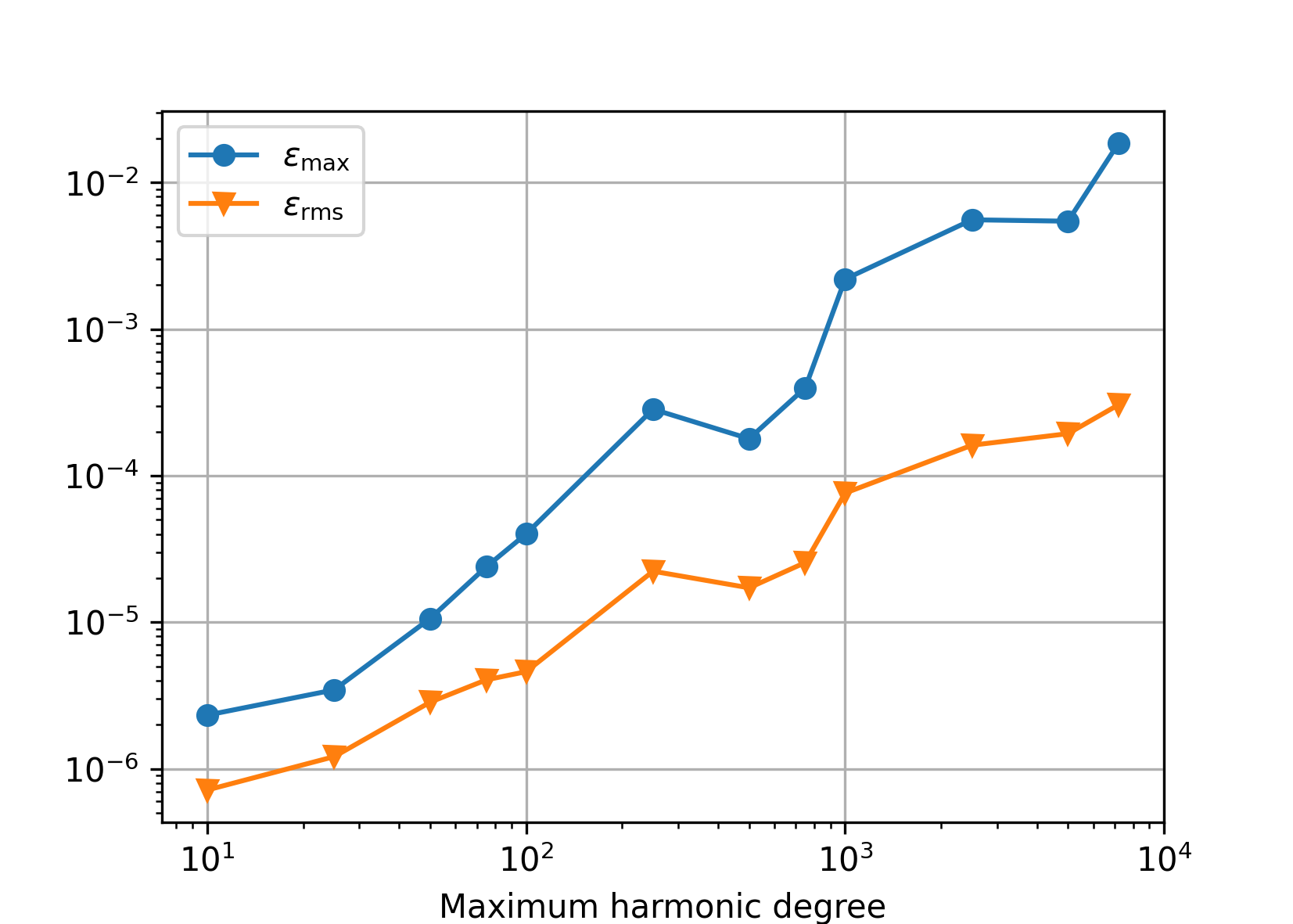
Accuracy

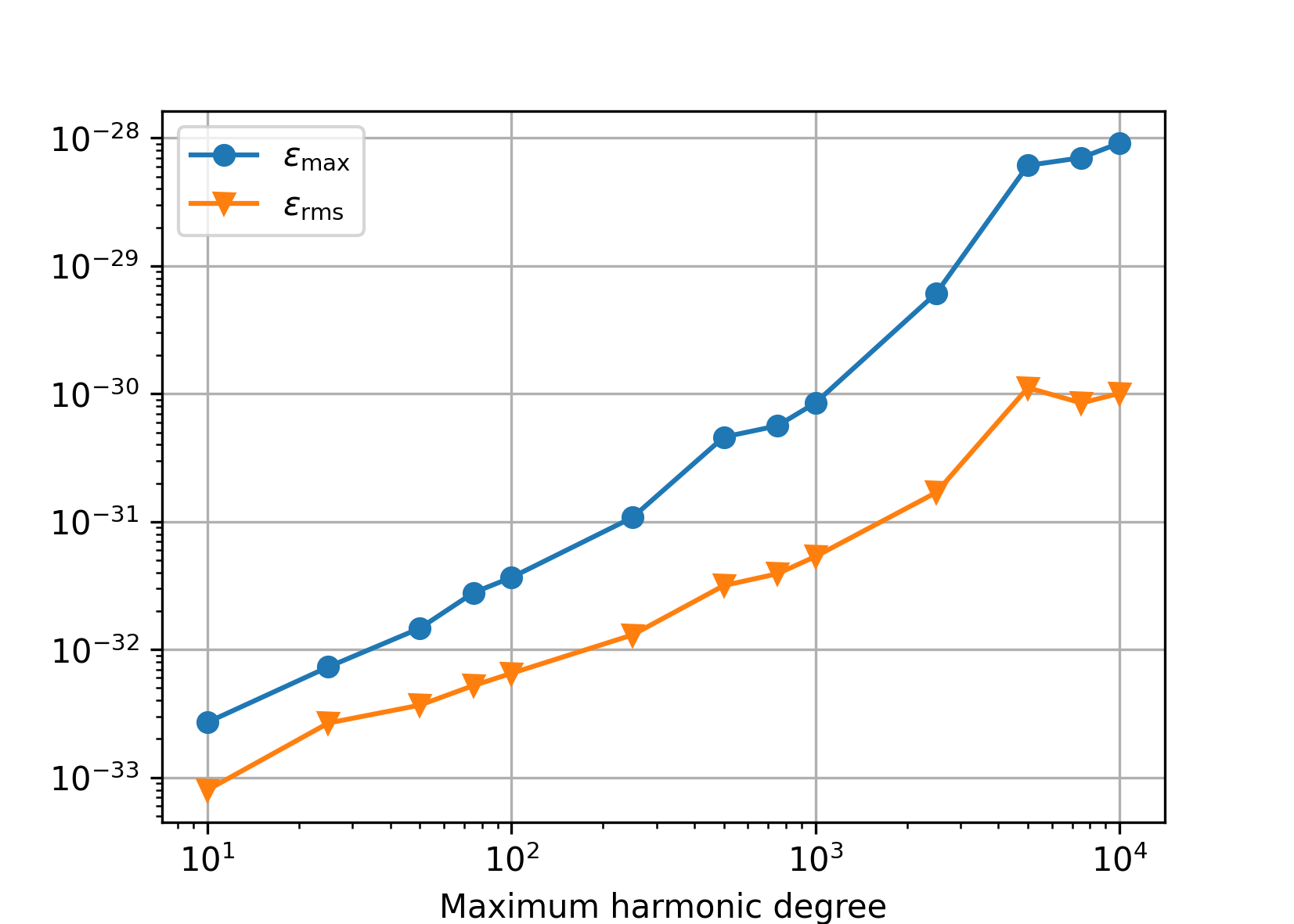
We generated reference random spherical harmonic coefficients from the interval [-1.0, 1.0] up to degree N, then synthesized the signal up to degree N, and, finally, harmonically analyzed the signal up to the same N degree. Below are plotted the following statistics obtained from the differences between the recovered and the reference coefficients:

• \(\varepsilon_{\max} = \max_{n,m}|\bar{Q}_{nm} - \bar{Q}^{(\mathrm{ref})}_{nm}|\),

• \(\varepsilon_\mathrm{rms} = \sqrt{\frac{2}{(N + 1) (N + 2)} \, \sum_{n,m} \left(\bar{Q}_{nm} - \bar{Q}^{(\mathrm{ref})}_{nm} \right)^2}\).

Single precision

In single precision, the tests are conducted up to N = 7200 only. Somewhere beyond that degree, it becomes difficult to compute the nodes of the Gauss–Legendre quadrature without an overflow in single precision. The Driscoll–Healy quadrature could be used as an alternative, but this would produce heterogeneous tests.

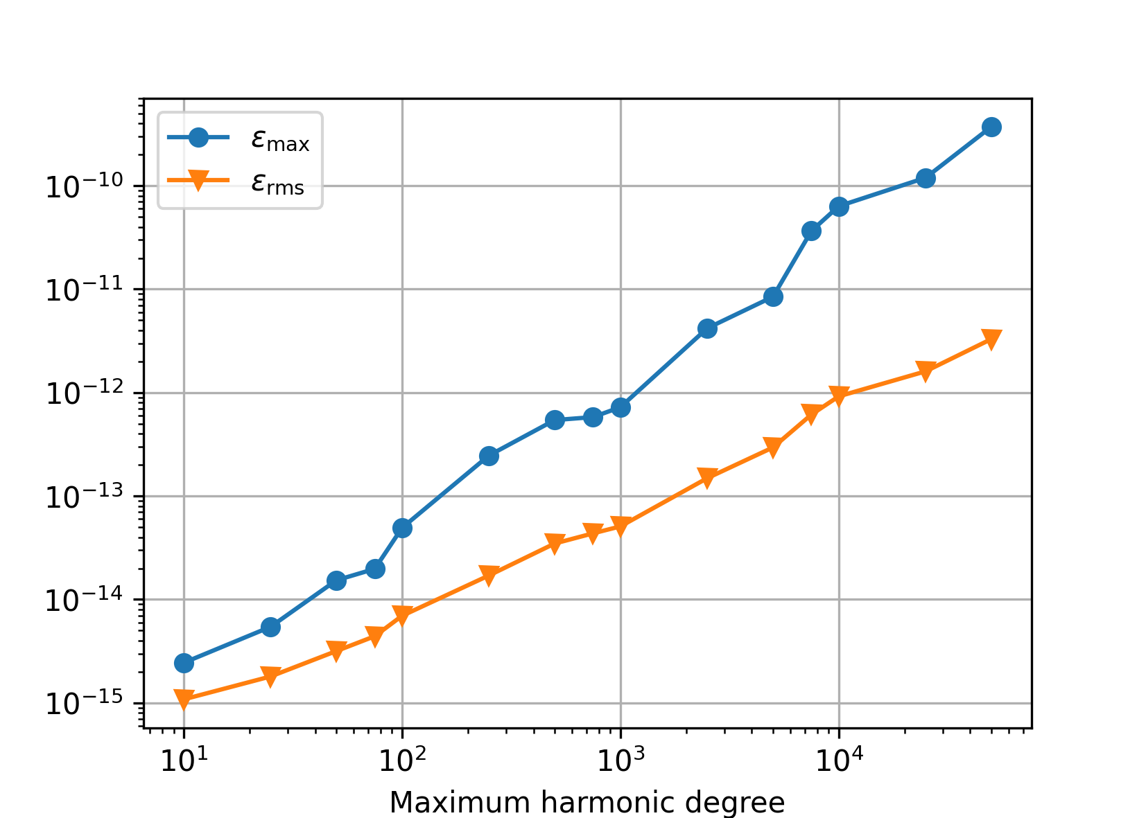
Double precision

Polar optimization disabled (default).

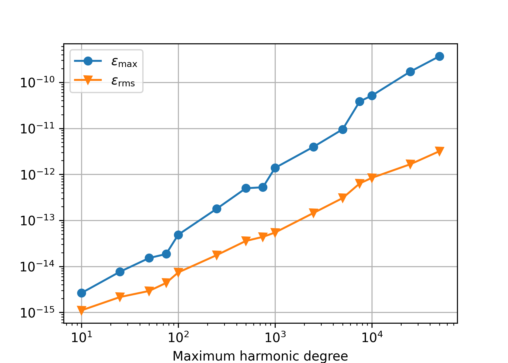
Polar optimization enabled (charm_glob_polar_optimization_a1 = 100, charm_glob_polar_optimization_a2 = 0.01). Comparing this figure and the previous one, it is seen that even though the polar optimization introduces approximations to spherical harmonic transforms, the numerical accuracy is the same. The small differences between the two figures are caused by the fact that a new set of random spherical harmonic coefficients was generated in both experiments.

Quadruple precision

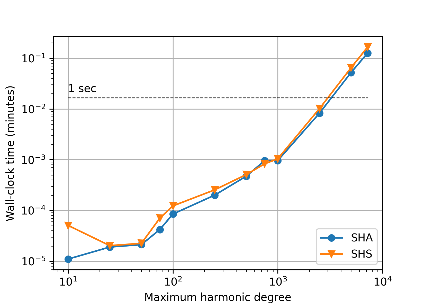
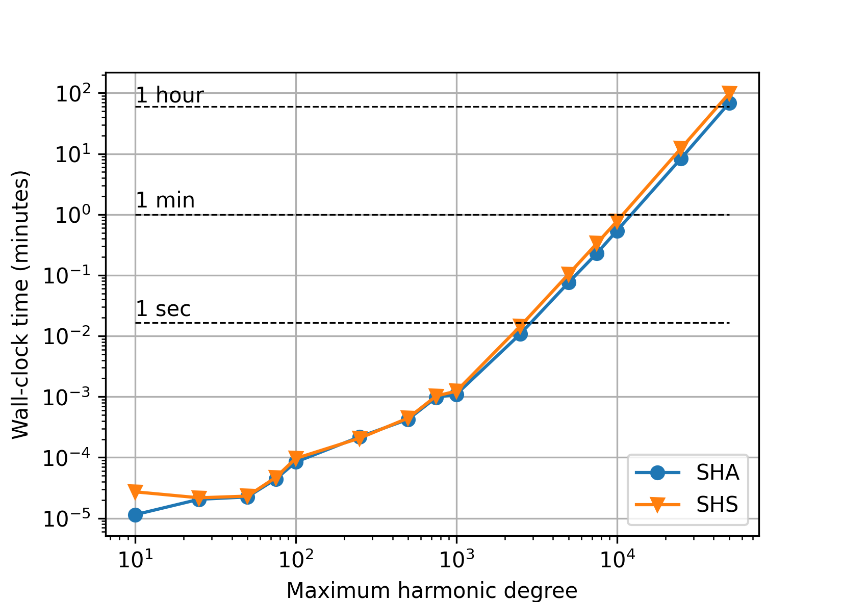
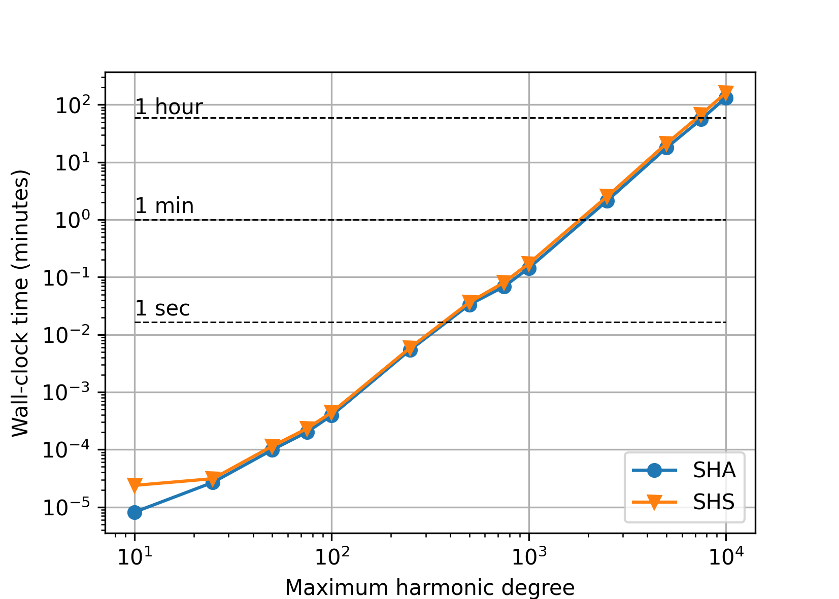
Speed

The figures that follow plot the wall-clock times needed to perform spherical harmonic synthesis and analysis in the experiments from the Accuracy section.

Single precision

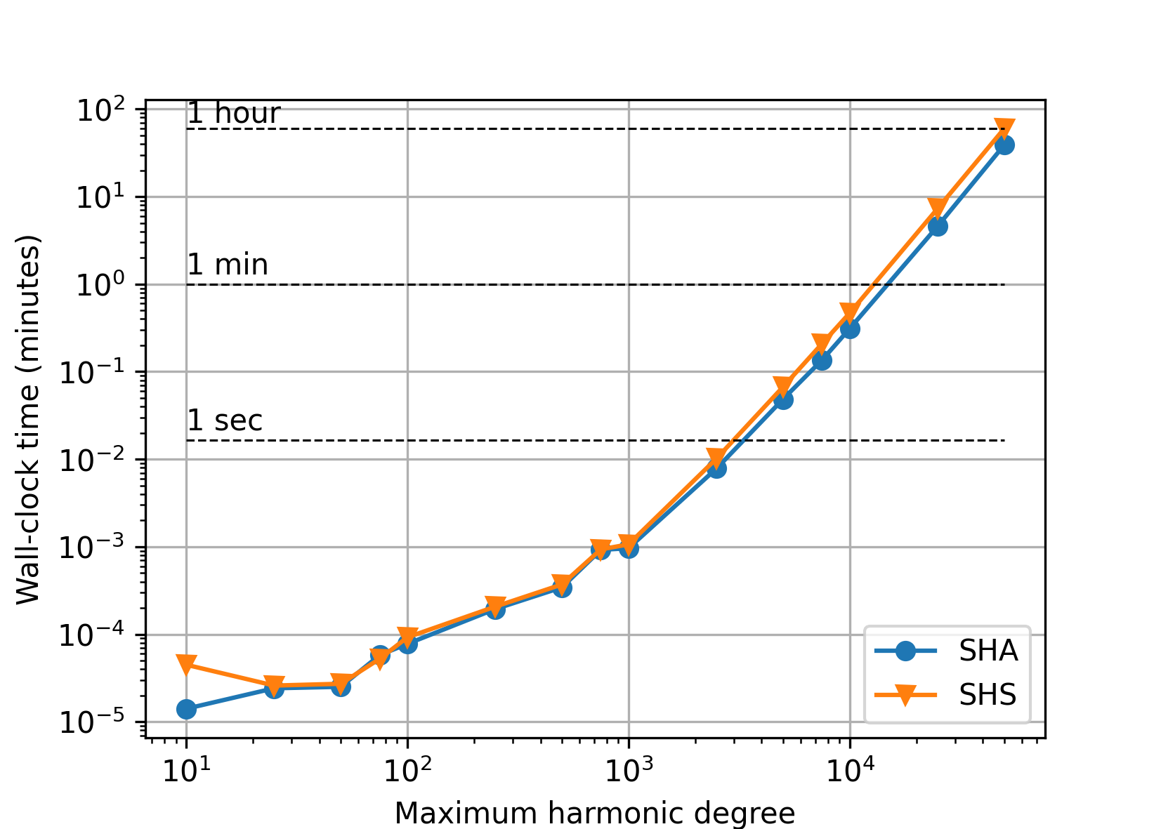
Double precision

Polar optimization disabled (default).

With the polar optimization enabled (charm_glob_polar_optimization_a1 = 100, charm_glob_polar_optimization_a2 = 0.01), the performance improved almost by 40 percent (depending on the maximum degree), while the accuracy remained the same (see Accuracy). More aggressive polar optimization can further improve the performance, but, after some critical point, only at the cost of deteriorated accuracy.

Quadruple precision

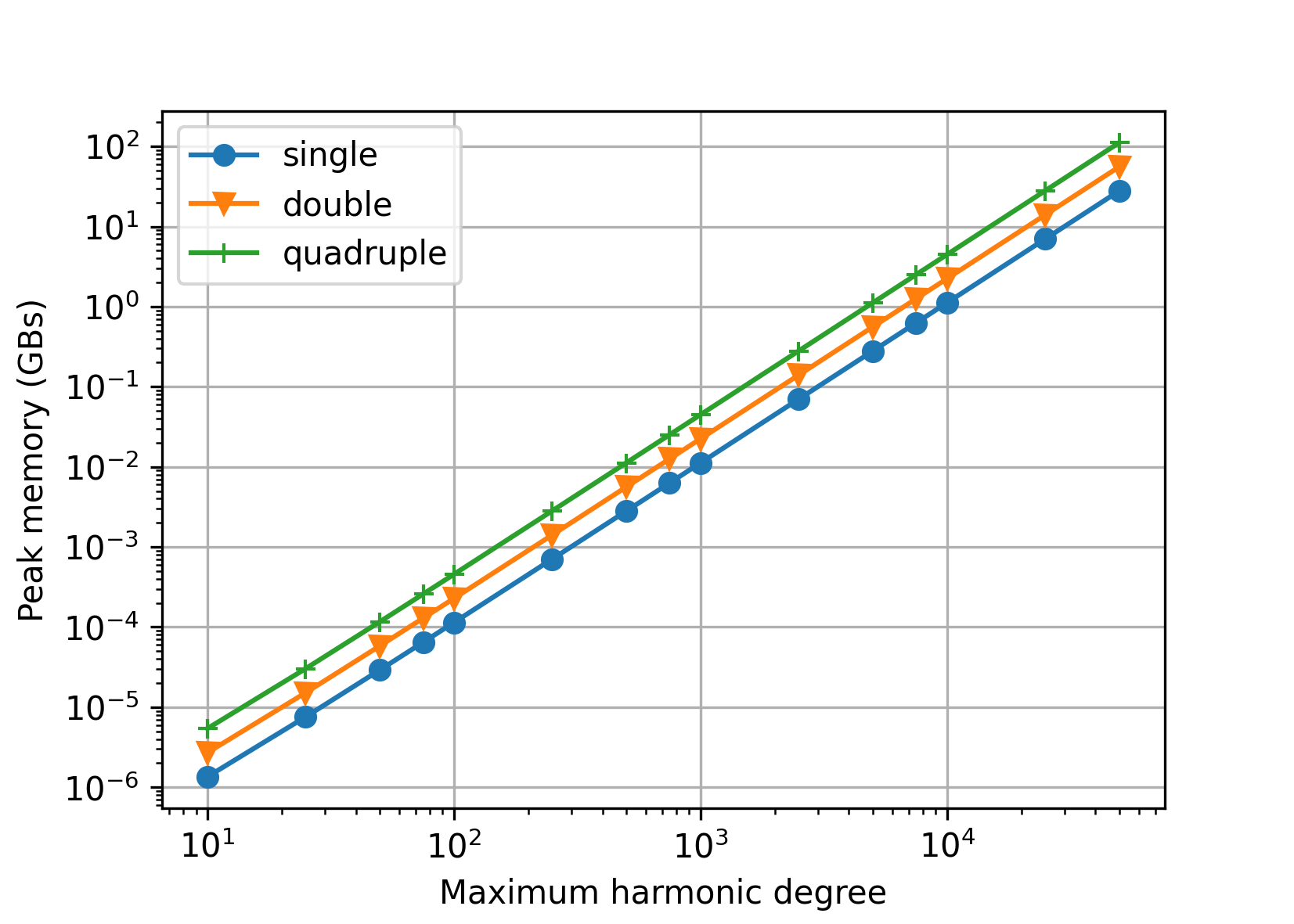
Memory

The next figure shows theoretical memory requirements for spherical harmonic analysis/synthesis of point data values sampled at the Gauss–Legendre grid. The values were computed for single, double and quadruple precision as (GBs)

\[\left((N + 1) \, (2 \, N + 2) + (N + 1)^2 \right) \, \frac{B}{1024^3}{,}\]

where

• \(N\) is the maximum harmonic degree, which determines the size of arrays to store the input data grid, \((N + 1) \, (2 \, N + 2)\), and the spherical harmonic coefficients, \({\sim}(N + 1)^2\), and

• \(B\) is the number of bytes needed to store a single float, double or __float128 floating point value (here assumed 4, 8 and 16 Bytes, respectively).

Although these are theoretical requirements, they model the reality very well, as all the remaining arrays are significantly smaller.