Some definitions to make things clear

Notation summary

Notation

Symbol	Meaning
\(\varphi \in \big[-\frac{\pi}{2}, \frac{\pi}{2} \big]\)	Spherical latitude
\(\theta \in \big[0, \pi \big]\)	Spherical co-latitude
\(\lambda \in \big[0, 2\pi \big)\)	Spherical longitude
\(r > 0\)	Spherical radius
\(n = 0, 1, 2, \dots\)	Spherical harmonic degree
\(m = 0, 1, 2, \dots, n\)	Spherical harmonic order
\(n_{\max} = \mathbb{N}_0\)	Maximum spherical harmonic degree of the expansion
\(P_n\)	Un-normalized Legendre polynomial of degree \(n\)
\(\bar{P}_{nm}\)	Fully-normalized associated Legendre function of the first kind of degree \(n\) and order \(m\)
\(P_{nmj}\)	Fourier coefficient of the fully-normalized associated Legendre function of degree \(n\) and order \(m\). \(j\) is a coefficient related to the wave-number \(k\) as \(j = \left[\frac{k}{2}\right]_{\mathrm{floor}}\)
\(\bar{Y}_{nm}\)	Real-valued \(4\pi\)-fully-normalized surface spherical harmonic of degree \(n\) and order \(m\)
\(\{ \bar{C}_{nm},\, \bar{S}_{nm} \}\)	Real-valued \(4\pi\)-fully-normalized surface spherical harmonic coefficients of degree \(n\) and order \(m\)
\(\mu\)	Scalling parameter of spherical harmonic coefficients (for instance, the geocentric gravitational constant)
\(R > 0\)	Radius of the reference sphere to which spherical harmonic coefficients refer to.
\(f\)	Real-valued function on the unit sphere
\(\tilde{f}\)	Mean value of a real-valued function \(f\) over a grid cell
\(\sigma\)	Unit sphere
\(\Delta \sigma\)	Area of a grid cell on the unit sphere

Evaluation points and evaluation cells

CHarm can work with evaluation points and evaluation cells.

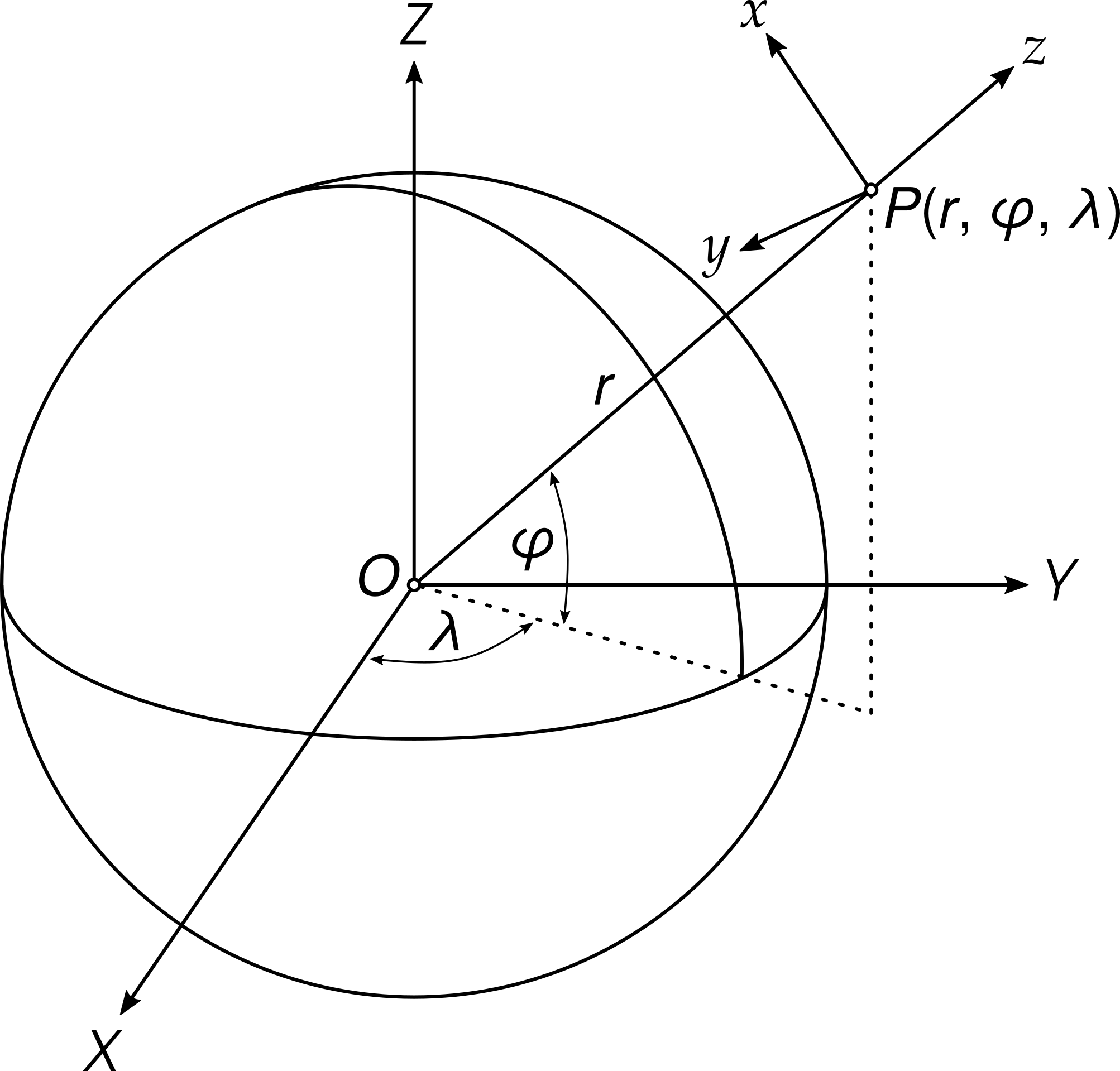
• An evaluation point is given by the spherical latitude, \(\varphi \in [-\frac{\pi}{2}, \frac{\pi}{2}]\), the spherical longitude, \(\lambda \in [0, 2\pi)\), and the spherical radius, \(r > 0\).

• An evaluation cell is given the minimum and the maximum latitude, \(\varphi^{\mathrm{min}}\) and \(\varphi^{\mathrm{max}}\), respectively, the minimum and the maximum longitude, \(\lambda^{\mathrm{min}}\) and \(\lambda^{\mathrm{max}}\), respectively, and a single spherical radius \(r\) that is constant over the cell.

Occasionally, spherical co-latitude, \(\theta = \frac{\pi}{2} - \varphi\), \(\theta \in [0, \pi]\), will be used instead of the spherical latitude.

Note

Angular inputs/outputs (if any) must always be provided in radians in CHarm.

Evaluation points/cells can either be organized as a grid or as scattered points/cells.

• Grid of points is defined by

  • nlat latitudes over a single grid meridian,

  • nlon longitudes over a single grid latitude parallel, and

  • nlat spherical radii over a single grid meridian.

  The grid has in total nlat * nlon points. The spherical radius r may vary with the latitude, but is implicitly consider as constant in the longitudinal direction (hence the nlat number of radii).

  CHarm does not store all nlat * nlon grid coordinates, but only the grid boundaries to save some memory.

• Grid of cells is defined by

  • nlat minimum cell latitudes over a single grid meridian,

  • nlat maximum cell latitudes over a single grid meridian,

  • nlon minimum longitudes over a single grid latitude parallel,

  • nlon maximum longitudes over a single grid latitude parallel, and

  • nlat spherical radii over a single grid meridian.

  The grid has in total nlat * nlon cells. Given that the spherical radius (1) is implicitly constant over a grid cell and (2) may vary only with latitude, there is nlat spherical radii.

  Again, CHarm stores only the grid boundaries.

• Scattered points are defined by

  • nlat == nlon latitudes,

  • nlat == nlon longitudes, and

  • nlat == nlon spherical radii.

  The total number of scattered points is nlat == nlon.

• Scattered cells are defined by

  • nlat == nlon minimum latitudes,

  • nlat == nlon maximum latitudes,

  • nlat == nlon minimum longitudes,

  • nlat == nlon maximum longitudes,

  • nlat == nlon spherical radii.

  The total number of scattered cells is nlat == nlon.

Note

Routines implementing the definitions of evaluation points/cells are gathered in charm_crd and pyharm.crd.

Surface spherical harmonics

Real-valued surface spherical harmonics \(\bar{Y}_{nm}(\varphi, \lambda)\) of degree \(n\) and order \(m\) are defined as (e.g., Hofmann-Wellenhof and Moritz, 2005)

\[\begin{split}\bar{Y}_{nm}(\varphi, \lambda) = \bar{P}_{nm}(\sin \varphi) \begin{cases} \cos(m\, \lambda){,}\\ \sin(m\, \lambda){.} \end{cases}\end{split}\]

Here,

\[\begin{split}\bar{P}_{nm}(\sin \varphi) = \begin{cases} \sqrt{(2n + 1)} \, P_n(\sin\varphi){,} &m = 0 {,}\\ \sqrt{2 (2n + 1) \dfrac{(n - m)!}{(n + m)!}} \, \left(1 - \sin^2\varphi\right)^{m / 2} \, \dfrac{\mathrm{d}^m P_n(\sin\varphi)}{\mathrm{d} (\sin\varphi)^m} {,} \quad &0 < m \leq n {,} \end{cases}\end{split}\]

are the fully-normalized associated Legendre functions of the first kind and

\[P_n(\sin\varphi) = \dfrac{1}{2^n \, n!} \, \dfrac{\mathrm{d}^n}{\mathrm{d} (\sin\varphi)^n} \left(\sin^2\varphi - 1 \right)^n\]

are the (un-normalized) Legendre polynomials (\(m = 0\), so the order is omitted from the notation).

Warning

CHarm evaluates the latitudinal derivatives of Legendre functions by the fixed-order recurrences from Appendix A.1 of Fukushima (2012b), which are singular at the poles.

Note

Applied is the geodetic \(4\pi\) full normalization. Neither other normalizations nor complex spherical harmonics are supported (yet?).

Note

The numerical evaluation of Legendre functions is performed after Fukushima (2012a), so spherical harmonics can be safely evaluated up to high degrees and orders (tens of thousands and even well beyond).

Spherical harmonic analysis

Assume a harmonic function \(f(r, \varphi, \lambda)\) given on a sphere with the radius \(r\). By surface spherical harmonic analysis,

\[\begin{split}\left.\begin{aligned} \bar{C}_{nm} \\ \bar{S}_{nm} \end{aligned}\right\} = \dfrac{1}{4 \pi} \, \dfrac{R}{\mu} \, \left( \dfrac{r}{R} \right)^n \displaystyle\iint_{\sigma} f(r, \varphi, \lambda) \, \bar{Y}_{nm}(\varphi,\lambda) \, \mathrm{d}\sigma {,}\end{split}\]

it is possible to compute its spherical harmonic coefficients \(\{ \bar{C}_{nm},\, \bar{S}_{nm} \}\). The coefficients are normalized by the \(\mu\) constant and, if \(r \neq R\), they are additionally rescaled from the data sphere with the radius \(r\) to the reference sphere with the radius \(R\).

• If \(r = R = \mu = 1\), one arrives at the surface spherical harmonic analysis that is well-known from the literature.

• If \(r = R\), then \(f\) does not even have to be harmonic.

• In geosciences, \(\mu\) frequently represents the geocentric gravitational constant and \(R\) stands for the equatorial radius of the Earth.

If \(f\) is band-limited (that is, it has a finite spherical harmonic expansion) and is sampled at suitable grid points, these equations can be computed rigorously (analytically). Examples of such quadrature, employed in CHarm, are the Gauss–Legendre quadrature (Sneeuw, 1994) and the Driscoll–Healy quadrature (Driscoll and Healy, 1994).

In CHarm, the coefficients can also be computed from mean values \(\tilde{f}\) of \(f\) given over grid cells. In that case, however, the quadratures are no longer exact.

Note

Routines for spherical harmonic analysis are gathered in charm_sha and pyharm.sha.

Spherical harmonic synthesis

Assume that surface spherical harmonic coefficients \(\{ \bar{C}_{nm},\, \bar{S}_{nm} \}\) of a harmonic function \(f(r, \varphi,\lambda)\) are available up to degree \(n_{\mathrm{max}}\) and are scaled to a constant \(\mu\) and a reference sphere with the radius \(R\). Then, it is possible to reconstruct a point value of \(f(r, \varphi,\lambda)\) for any \((r > R, \varphi,\lambda)\) exactly by solid spherical harmonic synthesis,

\[\displaystyle f(r, \varphi,\lambda) = \frac{\mu}{R} \, \sum_{n = 0}^{n_{\max}} \left( \frac{R}{r} \right)^{n + 1} \, \sum_{m = 0}^{n} \left( \bar{C}_{nm}\, \cos(m \, \lambda) + \bar{S}_{nm} \, \sin(m \, \lambda) \right) \, \bar{P}_{nm}(\sin\varphi){.}\]

If the evaluation points \((r, \varphi,\lambda)\) form a grid (as defined in Evaluation points and evaluation cells), highly efficient FFT-based algorithms can be employed (e.g., Colombo, 1981; Sneeuw, 1994; Jekeli et al, 2007; Rexer and Hirt, 2015). CHarm takes advantage of these algorithms in order to achieve efficient grid-wise numerical computations.

In addition to point values of \(f\), CHarm computes also mean values of \(f\) over cells (as defined in Evaluation points and evaluation cells):

\[\displaystyle \tilde{f}(r, \varphi_{\mathrm{min}},\varphi_{\mathrm{max}}, \lambda_{\mathrm{min}},\lambda_{\mathrm{max}}) = \frac{1}{\Delta \sigma} \int\limits_{\varphi = \varphi_{\mathrm{min}}}^{\varphi_{\mathrm{max}}} \int\limits_{\lambda = \lambda_{\mathrm{min}}}^{\lambda_{\mathrm{max}}} f(r, \varphi,\lambda) \, \mathrm{d}\lambda \, \cos\varphi \, \mathrm{d} \varphi\]

and

\[\begin{split}\displaystyle \tilde{f}(r(\varphi, \lambda), \varphi_{\mathrm{min}}, \varphi_{\mathrm{max}}, \lambda_{\mathrm{min}},\lambda_{\mathrm{max}}) =& \frac{1}{\Delta \sigma} \int\limits_{\varphi = \varphi_{\mathrm{min}}}^{\varphi_{\mathrm{max}}} \int\limits_{\lambda = \lambda_{\mathrm{min}}}^{\lambda_{\mathrm{max}}} f(r(\varphi,\lambda), \varphi,\lambda) \\ &\times \mathrm{d}\lambda \, \cos\varphi \, \mathrm{d} \varphi {,}\end{split}\]

where \(\Delta\sigma\) is the size of the cell on the unit sphere.

Note that in the latter equation, \(f(r(\varphi,\lambda),\varphi,\lambda)\) is defined on an irregular surface given by a spherical radius \(r(\varphi,\lambda)\) that varies with the latitude and longitude. This computation is unique to CHarm and cannot be found in any other publicly available package or library.

Note

Routines for spherical harmonic synthesis are gathered in charm_shs and pyharm.shs.

Local north-oriented reference frame

Local north-oriented reference frame (LNOF) is the right-handed Cartesian coordinate system defined as follows: the origin is at the evaluation point \(P(r, \varphi, \lambda)\), the \(x\)-axis points to the north, the \(y\)-axis points to the west and the \(z\)-axis points radially outwards. At \(P(r, \varphi, \lambda)\), the \(xy\) plane is tangential to the sphere with the radius \(r\) passing through \(P(r, \varphi, \lambda)\).

References

• Colombo OL (1981) Numerical methods for harmonic analysis on the sphere. Report No. 310, Department of Geodetic Science and Surveying, The Ohio State University, Columbus, Ohio, 140 pp

• Driscoll, J. R., Healy, D. M. (1994) Computing Fourier transforms and convolutions on the 2-sphere. Advances in Applied Mathematics 15:202-250

• Fukushima T (2012a) Numerical computation of spherical harmonics of arbitrary degree and order by extending exponent of floating point numbers. Journal of Geodesy 86:271–285, doi: 10.1007/s00190-011-0519-2

• Fukushima T (2012b) Numerical computation of spherical harmonics of arbitrary degree and order by extending exponent of floating point numbers: II first-, second-, and third-order derivatives. Journal of Geodesy 86, 1019–1028, doi: 10.1007/s00190-012-0561-8

• Hofmann-Wellenhof B, Moritz H (2005) Physical Geodesy. Springer, Wien, New York, 403 pp

• Jekeli C, Lee JK, Kwon JH (2007) On the computation and approximation of ultra-high-degree spherical harmonic series. Journal of Geodesy 81:603–615, doi: 10.1007/s00190-006-0123-z

• Rexer M, Hirt C (2015) Ultra-high-degree surface spherical harmonic analysis using the Gauss–Legendre and the Driscoll/Healy quadrature theorem and application to planetary topography models of Earth, Mars and Moon. Surveys in Geophysics 36:803–830, doi: 10.1007/s10712-015-9345-z

• Sneeuw N (1994) Global spherical harmonic analysis by least-squares and numerical quadrature methods in historical perspective. Geophysical Journal International 118:707–716